 9.3. Types of Splines 9.3. Types of Splines
 The Bezier Curve was pioneered by P.Bezier for computer modelling of surfaces for the design of automobiles. In fact Renault have used his UNISURF system (which uses the Bezier Curve method) on several of the vehicles.
The key the Beziers method is the use of blending functions. These affect the behaviour of the curve from four control points. The four blending functions represent the 'influence' each control point has on the curve.
There are several drawbacks in using this method. The blending functions affect all points along the curve. In other words, it does not have localised control over the curve. Also, the number of control points affected the degree of the curve. The higher the degree, the higher the lack of control over the curve there was.
It is simple to use a Bezier curve to get a Bezier surface. The Bezier surface is just a mesh of Bezier curves anyway. Obviously there are lots of similarities between them.
There are two characteristics of Bezier surfaces that are important to remember while designing them.
(1)
The surface passes through the four corner control points
of the surface control net.
(2)
The surface tangent in both the u and v direction at each
corner control point passes through each of the adjacent
edge control points. In other words, the tangent is
defined by the corner control point and the adjacent edge
control point
(see Fig. 9.1)
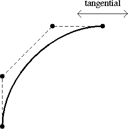
Fig. 9.1 : Bezier surface characteristics
These two are considered most important when surfaces are
to be joined together. To get a smooth seemless join, the shared
control point and the two internal control points either side in
each patch of adjoining surfaces should be colinear
(see Fig. 9.2)
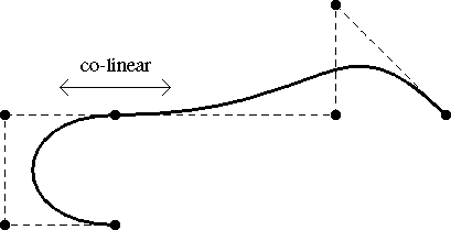
Fig. 9.2 : Joining Bezier surfaces
These are some example object types and how to build them out of Bezier surfaces.
9.3.1.3.1. Volumes of revolution
One thing that Bezier surfaces are good for is modeling volumes of revolution. Sketch the profile of the object and draw in the control points for a series of Bezier curves that would match it. These become the edges of a series of Bezier surfaces that will be used to model a quarter of the revolution.
Imagine these edges are in the x-z plane and the profile is to be revolved 90 degrees about the z axis. Lets just take one of the control points. Its x and z coordinates are just the distances from the respective axis, and the y coordinate is 0. The control point on the opposite side of the resultant surface will be in the y-z plane. Its z coordinate is the same, and the x and y coordinates are swapped.
Now we need to work out the coordinates of the two internal
control points of this row of the surface. The tangents at the
axis need to be perpendicular so that all the surfaces of the
revolution join seemlessly. So it turns out that the internal
control points are just shifted away from the axis. For a
circular sweep, the distance is roughly 0.55 times the distance
of the edge control points from the z axis.
The coordinates for the other three quarters of the revolution are easily calculated by just mirroring and swapping about the ones just worked out.
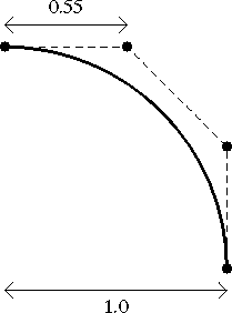
Fig. 9.3 : Bezier approx. of quarter circle
Tubes are constructed in two symmetrical halves; each a
surface. The edge control points are on opposite sides on the
surface of the tube. The internal control points are just shifted
out again so the tangents at the top and bottom are
perpendicular. For a circular cross section the distance away
from the centre line is about 0.63 times the height of the tube.
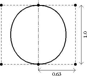
Fig. 9.4 : Bezier approximation of cylinder
This is a simple example of how two Bezier surfaces can be
used to model a convex lens. Below is some data used to model the
lens. The first block of numbers is the coordinates of the
control points, and the second is the control point numbers for
the two surfaces. The line numbers are just for easy reference.
    1:     -1     0     0

    2:     -1    -0.55  0

    3:     -0.55 -1     0

    4:      0    -1     0

    5:     -1     0.55  0

    6:     -0.55  0     0.5

    7:      0    -0.55  0.5

    8:      0.55 -1     0

    9:     -0.55  1     0

   10:      0     0.55  0.5

   11:      0.55  0     0.5

   12:      1    -0.55  0

   13:      0     1     0

   14:      0.55  1     0

   15:      1     0.55  0

   16:      1     0     0

   17:     -0.55  0    -0.5

   18:      0    -0.55 -0.5

   19:      0     0.55 -0.5

   20:      0.55  0    -0.5


           1 2 3 4 5 6 7 8 9 10 11 12 13 14 15 16

           1 2 3 4 5 17 18 8 9 19 20 12 13 14 15 16
Figure 9.1 shows the lens control net from above. The x axis goes off to the right, and the y axis goes up the page. Notice that we only needed four extra control points for the second/bottom surface because all the edge ones can be shared with the first/top surface.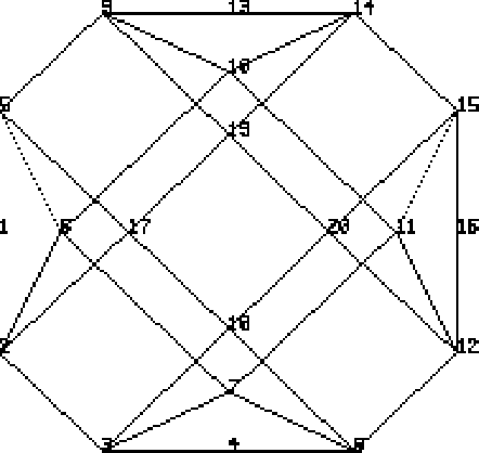
Fig. 9.1 : Lens - Control net from above
Figure 9.2 shows the two surfaces from the side.
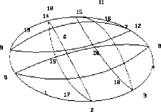
Fig. 9.2 : Lens - Surfaces from side
This is an example of a more complex object modeled with
Bezier surfaces; a teapot. Because it is constructed from 306
control points and 32 surfaces the data has not been included
here. The body and lid are just volumes of revolution. The spout
and handle are bent tubes.
Figure 9.1 shows the control nets for the Bezier surfaces. If you look carefully at the back corner, you can see a bug in the geometry definition. One of the control point numbers for that surface was typed in twice.
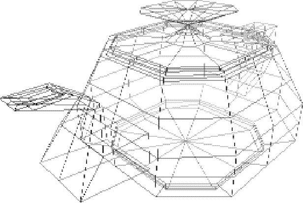
Fig. 9.1 : Teapot - Control nets
Figure 9.2 shows the surfaces themselves.
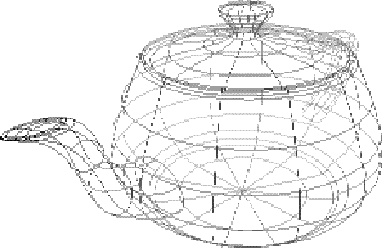
Fig. 9.2 : Teapot - Surfaces
The natural starting point for a study of spline functions is the cubic spline because it is similar to the draftman's spline. It is a continuous cubic polynomial that interpolates the control points ( joints ). The polynomial coefficients for cubic splines are dependent on all n control points, their calculation involves inverting an (n+1) by (n+1) matrix. This has two disadvantages: (i) moving any one control point affects the entire curve, and (ii) the computation time needed to invert the matrix can interfere with rapid interactive reshaping of a curve.
B-Spline (which means Basis Spline) was the earliest spline method. It overcame the problems encountered by the Bezier Curve , by providing a set of blending functions that only had effect on a few control points. This gave the local control that was lacking.
Also, the problem of piecing curves together was avoided by allowing only those curves that possessed the required continuity at the joints. Most other spline techniques provided this at the loss of local control.
The overall formulation is much like that of the Bezier, but the key difference is in the formulation of the blending functions. The important feature of the B-Spline blending functions is that they are non-zero in only a small portion of the range of the particular parameter.
B-Spline share many of the advantages of Bezier Curves, but the main advantage is the local control of the curve shape. B- Splines also reduce the need to piece many curves together to define the final shape. Control points can be added at will without increasing the degree of the curve, thereby retaining the control over the curve that wouls be lost with a Bezier curve.
There are three types of B-splines: uniform nonrational B- splines, nonuniform nonrational B-splines and nonuniform rational B-splines. (Foley and et.al., 1987)
The term uniform means that the joints (knots) are spaced at equal intervals of the parameter t.
The term rational is used where x(t), y(t) and z(t) are each defined as the ration of two cubic polynomials.
B-splines consist of curve segments whose polynomial coefficients depends on just a few control points. This is called local control. In other words, moving a control point affects only in the region near the control point of a curve. In addition, the time needed to compute the coefficients is greatly reduced. B-splines have the same continuity as cubic splines, but do not interpolate their control points.
Nonuniform nonrational B-splines permit unequal spacing between the knots. These curves have several advantages over uniform B-splines.
First, continuity at selected join points can be reduced from second derivative (C2) to first derivative (C1) to C0 to none. If the continuity is reduced to C0, then the curve interpolates a control point, but without the undesirable effect of uniform B-splines, where the curve segments on either side of the interpolated control point are straight lines.
Also, starting and ending points can be easily interpolated exactly, without at the same time introducing lineat segments.
It is possible to add an additional knot and control point to nonuniform B-splines, so the resulting curve can be easily reshaped, whereas this cannot be done with uniform B-splines.
NURBS are Non-Uniform Rational B-Splines and is the term given to curves that are defined on a knot vector where the interior knot spans are not equal. As an example, we may have interior knots with spans of zero. Some common curves reqiure this type of non-uniform knot spacing. The use of this option allows better shape control and the ability to model a larger class of shapes.
Nonuniform rational B-splines (NURBS) are useful for two reasons. The first and most important reason is that they are invariant under perspective transformations of the control points.
A second advantage of rational splines is that they can define precisely any of the conic sections. A conic can be only approximated with nonrationals, by using many control points close to the conic.
Beta-splines is a tool for designing parametrically defined curves because they are tailored to geometric continuity rather than to parametric continuity. Geometric continuity is an intrinsic measure of continuity appropiate for spline development. It has been shown to be a relaxed form of parametric continuity independent of the parameterizations of the curve segments under consideration, but still sufficient for geometric smoothness of the resulting curve. However, geometric continuity is appropriate only for applications where the particular parameterization used is unimportant, since parameteric discontinuities are allowed. (Goodman and Unsworth, 1986)
Uniformly shaped Beta-splines are considered in which the bias and tension parameters are fixed throughout the length of the curves. Therefore, the extra control gained is not of a local nature, since a change in either parameter affected the entire curve.
V-spline curves, similar in mathematical structure to Beta- splines, are developed as a more computationally efficient alternative to splines in tension.
Although the splines in tension can be modified to allow tension to be applied at each control point, the procedure is computationally expensive. The v-spline curve uses more computationally tractable piecewise cubic curves segments, resulting in curves that are just smoothly joined as those of a standard cubic spline. (Nielson, 1986)


