 14. Transformations.
  14. Transformations.
 Three basic transformations:

Translation of point:
(x,y) --> (x+Tx,y+Ty)
same scale same orientation
Scale:
(x,y) --> (Sx*x, Sy*y)
same origin same orientation
Rotation:
(x,y) --> (x*cos-y*sin
, x*sin
+y*cos
)
rotate point anticlockwise throughdegrees
same origin same scale.


Example: Assume we have a graphics box.
(1) Rotate it through -90 degrees
(2) Shift it up by ten units
(3) Scale it by a factor of 2.
Look at origin (0,0) and point (10,10) and see how they are affected.
(1) (0,0)(0,0)
(10,10)(10*cos(-90) - 10sin(-90), 10*sin(-90) + 10*cos(-90))
(10cos(90) + 10sin(90), -10sin(90) + 10cos(90))
(10,-10)
(2) (0,0)(0,10)
(10,-10)(10,0) Note we use the new co-ordinates
(3) (0,10)(0,20) Scale x and y
(10,0)(20,0) use new co-ordinates from last transformation.


We represent a point (x,y) as [x y 1]

This vector can then be manipulated by matrices which represent the basic transformations. It is important to understand matrix multiplication and the order in which the matrix multiplication is carried out.
To translate a point:
 We can check the result of this by multiplying our vector with
this matrix.

 [ x y 1 ] .
            =====> [x+Tx y+Ty 1 ]


and again to check our result we multiply our vector.

 [ x y 1 ] .
            =====> [x*Sx y*Sy 1 ]


[ x y 1 ] .
=====> [x*Cos- y*Sin
x*Sin
+y*Cos
1 ]


 1 0 0
1 0 0 
 2 0 0
2 0 0 
 0 -1 0
T=  0 1 0
0 1 0  S=
S=  0 2 0
0 2 0  R=
R=  1 0 0
1 0 0 
 0 10 1
 0 0 1
0 0 1 
 0 0 1
0 0 1 

Therefore the entire transformation matrix is

 0 -1 0
 1 0 0
1 0 0 
 2 0 0
2 0 0 
 1 0 0
1 0 0  .
.  0 1 0
0 1 0  .
.  0 2 0
0 2 0  == R.T.S
 0 0 1
0 0 1 
 0 10 1
 0 0 1
0 0 1 
 0 -1 0
 2 0 0
2 0 0 
 1 0 0
1 0 0  .
.  0 2 0
0 2 0  == Temp.S
 0 10 1
 0 0 1
0 0 1 
 0 -2 0
 2 0 0
2 0 0  == Total Transformation Matrix.
 0 20 1


 0 -2 0
[ 0 0 1 ] .  2 0 0
2 0 0  == [ 0 20 1 ]
 0 20 1
 0 -2 0
[ 10 10 1 ] .  2 0 0
2 0 0  == [ 20 0 1 ]
 0 20 1

We can write general procedures to handle these 3
transformations and then use them in our programs.

subprogram translate(tx,ty:real;a:real array[1..3,1..3]);
a[1,1]1.0; a[1,2]
0.0; a[1,3]
0.0;
a[2,1]0.0; a[2,2]
1.0; a[2,3]
0.0;
a[3,1]tx; a[3,2]
ty; a[3,3]
1.0;
end_subprogram_translate.


subprogram scale(sx,sy:real; a:real array[1..3,1..3]);
a[1,1]  sx; a[2,2]
  sy; a[3,3]
  1.0;
1.0;
a[1,3]  0.0; a[2,3]
  0.0; a[2,1]
  0.0;
0.0;
a[1,2]  0.0; a[3,1]
  0.0; a[3,2]
  0.0;
0.0;
end_subprogram_scale.


subprogram rotate(theta:real;a:real array[1..3,1..3]);
local real angle;
angle  theta * 2.0 * PI /360.0;
a[1,1]  cos(angle); a[2,2]
  cos(angle);
a[2,1]  -sin(angle); a[1,2]
  sin(angle);
a[3,1]  0.0; a[3,3]
  1.0;
1.0;
a[3,2]  0.0; a[1,3]
  0.0; a[2,3]
  0.0;
0.0;
end_subprogram_rotate.


subprogram multiply(a,b,c: real array[1..3,1..3]);
local integer i,j,k;
local real cij; {Used purely for efficiency .}
for i  1 to 3 do
for j  1 to 3 do
cij  0;
0;
for k  1 to 3 do
cij  cij + a[i,k] * b[k,j];
end for
c[i,j]  cij;
cij;
end for
end for
end_subprogram_multiply.

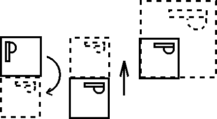
Consider the following transformation process:
What combination of translation, rotation and possibly scaling is needed to transform the left into the right?

Fig. 14.2 : Strange transformation.
Manipulation of three dimensional objects - (x,y,z) - also
use matrices: a 4x4 matrix for rotation, scaling and
translation. These may be multiplied together in a similar
fashion to 3x3.

Example:
An astroid (sic) has parametric equation
(R* cos^3(),R* sin^3(
))
Move it to (xc,yc) and rotate it anti-clockwise by theta degrees.
:
call rotate(theta,q);
call translate(xc,yc,p); {load up these matrices}
call multiply(q,p,r);
call myplot(radius,0.0,3);
theta0.0;
thetainc0.031415.....;
for i1 to 200 do
thetatheta + thetainc;
call myplot(radius* cos^3(theta),radius* sin^3(theta),2);
end for
:
subprogram myplot(x,y:real; n:integer);
global real array[1..3,1..3] r
call plot(r[1,1]*x + r[2,1]*y +r[3,1],
r[1,2]*x + r[2,2]*y +r[3,2], n)
return;
end_subprogram_myplot.


It is possible to use DDA techniques to generate
circles,ellipses etc as well as straight lines. The equation of a
circle is :

X2 + Y2 = R2 2xdx + 2ydy = 0
dy -x
=> -- = --
dx y
This leads to
Xn+1Xn +
Yn
Yn+1Yn -
Xn as before.


Xn+1Xn +
Yn
Yn+1Yn -
Xn+1

 small enough
1-
 2 ==1.

Yn+1-
Xn + (1-
2) Yn


[ Xn+1 Yn+1 1 ] = [ Xn Yn 1] .


Xn+1Xn*Cos(
) + Yn*Sin(
)
Yn+1Yn*Cos(
) - Xn*Sin(
) (if
clockwise)


